Customer Segmentation for Arvato Financial Services
Customer Segmentation report using machine learning models
Project Definition
project overview
This blog post is part of the Capstone Project for the Udacity Data Scientist nano degree program. In this project, the demographics data was utilized, to identify the potential customers for the mail-order company, a client of Arvato Financial Services. The supervised machine learning model, the outcome of this project, predicts whether or not individuals will respond to the campaign.
The blog post is composed of three parts:
-
Data Exploration: Understanding the data and data cleaning
-
Unsupervised learning: a customer segmentation report
-
Supervised learning: a classifier that predicts whether an individual will respond
project statement
In the first part, the main focus is on cleaning the data and exploring feature engineering options. With it completed, the data is then used to build an unsupervised machine learning model that performs segmentation for the customers and the general population. This model works to group individuals based on their features. By comparing to the general population, we could identify features that best describe the customers. Lastly, a prediction model was created to identify individuals who are more likely to respond to the campaign.
metrics
The prediction model is a binary classifier that separates the target group (who will respond) from the non-target group. As the dataset is highly imbalanced with a very low positive rate (1.2%), accuracy alone won’t be the appropriate evaluation metric to measure how well the model classifies the minority group. Instead, we will use the ROC AUC score to evaluate model performance. When evaluating this binary classifier, we like to capture all the positive groups while minimizing the false positive rate. ROC AUC score is, therefore, an appropriate metric, since it summarizes the trade-off between the true-positive rate and false-positive rate.
PART I: Data preparation
There are four data files associated with this project:
-
Udacity_AZDIAS_052018.csv: Demographics data for the general population of Germany; 891 211 persons (rows) x 366 features (columns).
-
Udacity_CUSTOMERS_052018.csv: Demographics data for customers of a mail-order company; 191 652 persons (rows) x 369 features (columns).
-
Udacity_MAILOUT_052018_TRAIN.csv: Demographics data for individuals who were targets of a marketing campaign; 42 982 persons (rows) x 367 (columns).
-
Udacity_MAILOUT_052018_TEST.csv: Demographics data for individuals who were targets of a marketing campaign; 42 833 persons (rows) x 366 (columns).
In addition to the above, Arvato provides two information files that describe attributes depicted in the data file.
-
DIAS Information Levels — Attributes 2017.xlsx: is a top-level list of attributes and descriptions, organized by informational category.
-
DIAS Attributes — Values 2017.xlsx: is a detailed mapping of data values for each feature in alphabetical order.
Feature summary — data exploration
As the first step, I created a feature summary file that summarizes the names of the attributes, the datatype, and missing or unknown representation. This summary file forms the basis of data preprocessing.
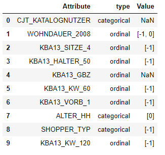 Screenshot of feature summary
A quick scan shows that the data in the file is mostly ordinal. For example, “D19_BANKEN_ANZ_12” describes the frequency of transaction activity. The values range from least frequent (0 = very low activity) to the most frequent (6 = very high activity). Since it is ranking based, the datatype “D19_BANKEN_ANZ_12” is ordinal. As most of the features are ordinal, I will pre-assign the feature type as ‘ordinal’. If further analysis shows otherwise, I will update the summary table.
In addition, it is noticed that the naming of most features follows a fixed structure. For example, in “D19_NAHRUNGSERGAENZUNG_RZ”, the first part “D19” presents the data source, while the rest describe the content of the feature (NAHRUNGSERGAENZUN = FOOD SUPPLEMENT). As data from the same source tend to be encoded in a similar manner, I decided to split the attribute names and use the first part (prefix) to investigate feature encoding in groups. By grouping the features, I was able to create a summary table for 276 features in a structured way.
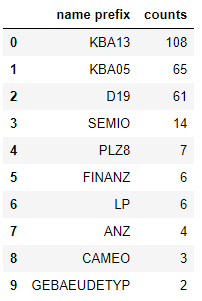 top-ranked prefixes used in naming
Furthermore, it is noticed from the analysis that:
-
Non-numeric values are assigned to a number of columns: “OST_WEST_KZ”, “CAMEO_DEUG_2015”, “CAMEO_DEU_2015”, “CAMEO_INTL_2015”, “D19_LETZTER_KAUF_BRANCHE”. I will therefore use LabelEncoder to transform it, and replace the abnormal values (“X”, “XX”) as unknowns.
-
‘EINGEFUEGT_AM’ uses date and time as feature values. I extracted the year from the string, which will be treated as numerical data.
-
As presented in the bar chart below, most of the features are ordinal, with few features are numerical. The rest, 73 features, is treated as categorical.
 Distribution of datatypes among the features
Data cleaning, transformation, and feature engineering
The data cleaning involves multiple steps:
-
Convert missing values to NaNs.
-
Drop rows and columns where a large portion are NaN’s
-
Replacing Missing values with the most frequent.
-
Outlier detection using Z-score
-
One Hot Encoding for Categorical Data.
-
Min-max scaling for ordinal and numerical data
-
Create a data cleaning pipeline, to be used later for later analysis
The data pre-processing pipeline includes two steps:
-
the first step ‘reduce dimension’ includes mapping the unknowns, selecting columns of interests, remove
-
the second step ‘combined pipe’ applies different data transformation strategies according to the datatypes.
At the first step, I decided to keep all the features in the analysis: the nan-threshold appears to cause data drain, which hampers the performance of the supervised machine learning model.
At the second step, the nan’s were replaced with either the median or the most frequent value. Afterward, the numerical values were scaled using MinMax scaler while the categorical values were transformed using OneHotEncoder.
PART II: Customer segmentation report
In this section, unsupervised learning techniques are utilized to compare the demographic data of the customers and the general population.
Principal Component Analysis
To start with, I used Principal Component Analysis (PCA) to summarize the information contained in the data files. This is an efficient way to combine similar features while maintaining the variance of the data.
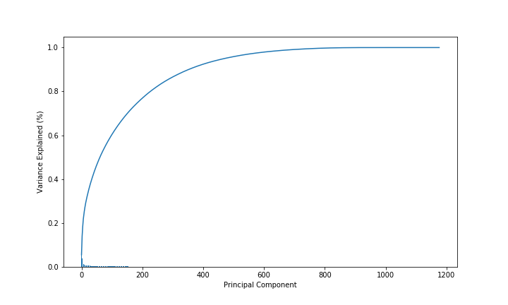
The accumulated explained variance increases, with the increase in the number of principal components included in the model. It was decided to include the first 216 PCA’s, which captures more than 80% of the accumulated variance.
Clustering
The clustering is based on the elbow method. I decided to include 10 clusters in total since additional clusters only slightly reduce the inertia of KNMeans.

Using the clustering model, I compared the difference between the customers and the general population. The figure below presents the distribution of the data over the 10 clusters. From the figures, it is concluded that customers tend to belong to cluster #2 and cluster #7, while the general population is evenly distributed among the clusters.
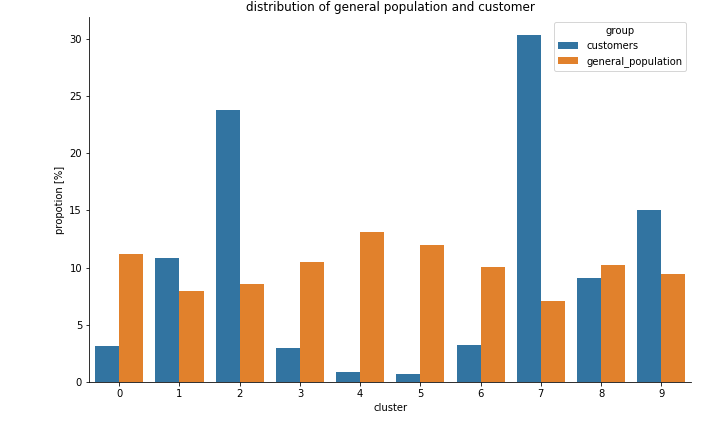
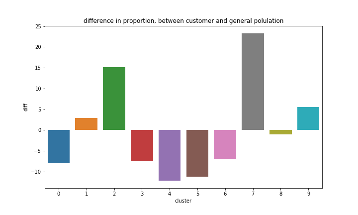
The bar chart above presents the difference between the general population and the customers, in terms of the proportion of each cluster. It is noticed that differences are the largest in cluster 5 and cluster 7.

The heatmap above presents the relevance of each PCA to each cluster. Combined with the comparison between the general population and customer, we could infer that potential customers tend to live in a neighborhood with a higher number of car ownership, and they are older than the general population.
PART III: Prediction
With segmentation completed, a supervised machine learning model was built to predict whether the individuals in the dataset will convert to be a customer. The analysis is based on demographics contained Udacity_MAILOUT_052018_TRAIN.csv (trainig data)and Udacity_MAILOUT_052018_TEST (test dta).csv. The training data contains one additional column named ‘response’ while we need to predict it for the testing dataset.
Training set:
total records: 42962
who responded to mail out campain: 532
who did not respond: 42430
na's in the RESPONSE column: 0
portion of response: 1.24%
A further examination shows that only 1.24% of people responded to the campaign in the training set, which results in a highly imbalanced data set. To deal with the imbalance dataset in this binary classification, I used the ROC AUC score to evaluate model performance that measures both the true positive and false-positive rates.
In modeling, I used Ensembling classifiers as it shows improved performances over a single learner. Besides, I made use of the balanced ensemble methods provided in [imbalanced-learn](https://imbalanced-learn.readthedocs.io/en/stable/index.html), which internally samples the data. As concluded in ref.[1], the balanced Ensembling classifier greatly enhances model performance.
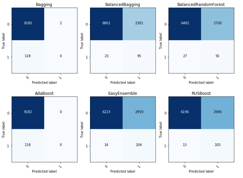 Confusion matrixes, using different classifiers
From the estimators that I compared, EasyEnsemble *was selected as it yielded the highest ROC AUC score. It yielded a ROC AUC score of 0.78, even without hyperparameter tuning. The non-balanced models (Bagging, AdaBoost) have a score of 0.5, which indicates the models failed to provide a prediction and all were predicted to be negative. In comparison, the balanced models show significantly improved performance, thanks to the balancing techniques internally implemented in *imbalanced-learn.
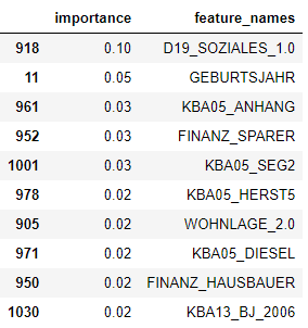 Feature importance
Figure about shows the feature importance. ‘D19_SOZIALES’ has the highest weight in the prediction model. A potential customer tends to have a value of ‘1.0 ’ in ‘D19_SOZIALES’. Unfortunately, the meaning of this feature was not provided in the information file. We were unable to further interpret the feature.
 Influence of the total number of features in ROC AUC score.
It however strikes me that the performance of the model is not highly dependent on the number of features used to create in the model. It already yields a ROC AUC score of 0.78, when including the top three of the most important features.
Further efforts were spared in fine-tuning the model, as provided below. From the parameters compared, it is decided to include 30 estimators for the base model and 30 estimators for the *EasyEnsembleClassifier. *The ROC AUC score is slightly increased to 0.80.
Conclusions
From the confusion matrix for EasyEnsemble, it is noted that the model has a true positive rate of 0.88. The classifier manages to identify the majority of the individuals who will respond. Even if we limit the campaign to the individuals who are predicted to be positive, we could still reach 88% of the target group (true positives). If adopting this strategy in the campaign, we could effectively reduce the campaign to 33% of its original size. In conclusion, the machine learning model works to predict whether or not each individual will respond to the campaign. The has the potential to help the mail-order company to better target the customers.
This is the first machine learning model that I created using real-world data. It is quite challenging a project in tow aspects:
-
The large dimension of the data set requires extensive efforts in understanding the data and establishing a strategy to process the data
-
It is also highly imbalanced, which requires proper sampling to be suitable for classification analysis.
The deeper that I dived into the data, the more I realized the importance of proper feature engineering. To enhance the performance of the data, I would refine the feature engineering strategies, to better select and extract information from the data set. Besides, I would also like to explore more advanced classifiers with enhanced performances in dealing with an imbalanced data set.
Reference:
[1].Comparison of ensembling classifiers internally using sampling: https://imbalanced-learn.readthedocs.io/en/stable/auto_examples/ensemble/plot_comparison_ensemble_classifier.html#sphx-glr-auto-examples-ensemble-plot-comparison-ensemble-classifier-py